But regardless of which category you fall into, you’re going to have to deal with Excel at some point. Marketers encounter tons of data every day – most of it very unorganized.

Excel can help you make sense of it, and in the right hands, Excel is a powerful tool for organizing overwhelming bulks of data.
These advanced Excel tricks and tips can help you become a better marketer.
Important: Before starting, define your goal
There’s no sense in doing fancy Excel tricks if you don’t have your end goal in mind. Before you start working on a big Excel sheet, define how you want the data to look at the end of the process.
For example, when if you want to produce a table, define which columns you want to see at the end of the process:

Or if you want to show charts, try to think what data you want to show and how:

Understanding your end goal makes it easier for you to understand how to get there using these tips.
Excel Trick 1: Concatenate or “&”
The Concatenate Function helps you join the content of multiple cells into one cell.
When should I use Concatenate?
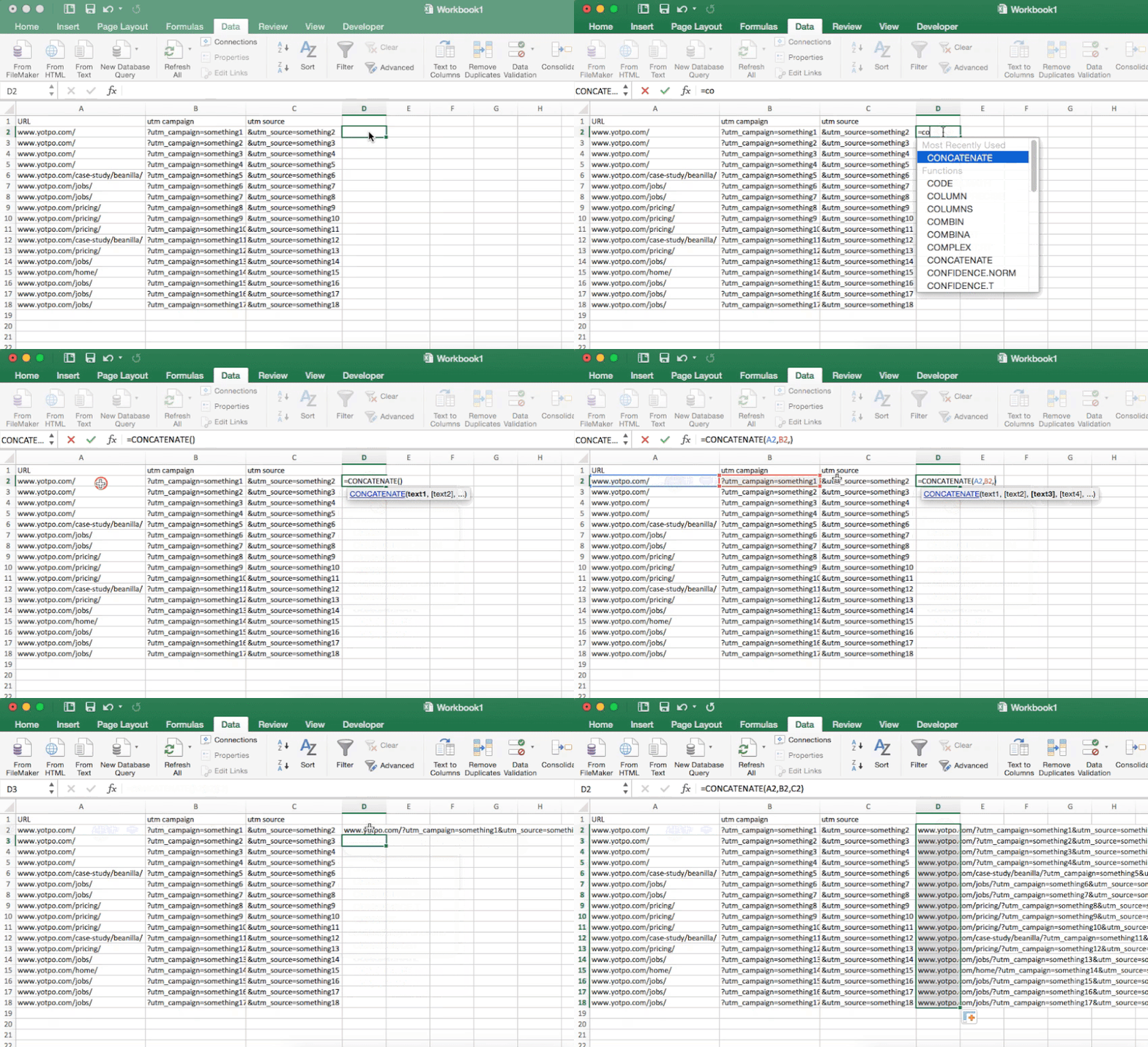
If you have an Excel sheet where the UTM Source, Medium and Campaign are in separate columns and you want to create a column that contains your full link with UTM tags, you can use Concatenate to do it easily.
How can I use Concatenate?
There’s 2 options for how to use this function:
You can use the classic CONCATENATE function.
Example: =CONCATENATE(A1,B1,C1)
Or you can just use “&” between the cells you want to join together.
Example: =A1&B1&C1
The content doesn’t have to be in a cell to add it with Concatenate – you can manually input the content into the Concatenate function.
Example: =CONCATENATE(A1,”utm_campaign”,B1)
Excel Trick 2: Text to Columns
This function makes it incredibly easy separate the content of a single Excel cell into multiple different cells.
When should I use Text to Columns?
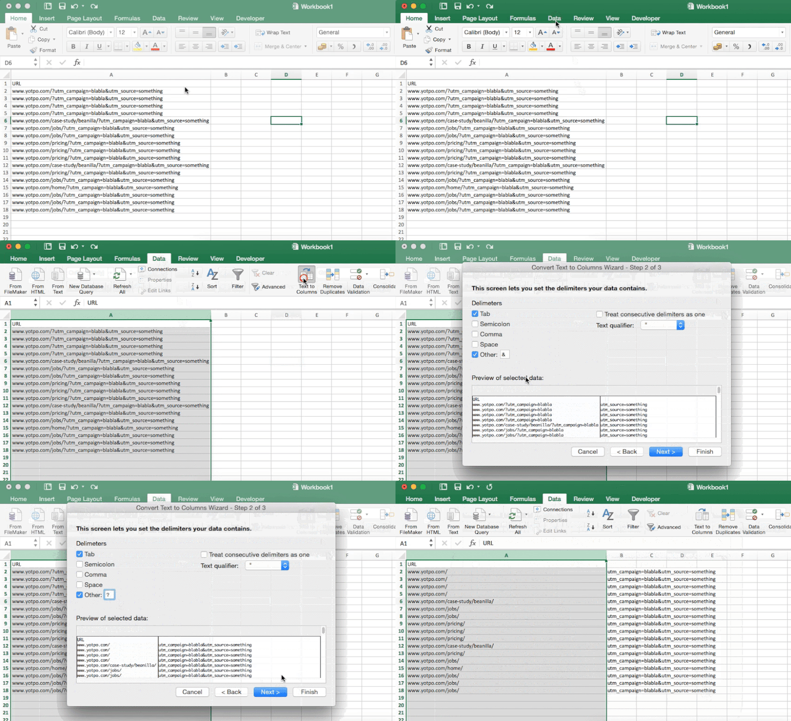
Let’s say you have a column that contains link with UTM tags. You can use Text to Columns to separate the link into 4 different columns for URL and UTM Source, Campaign and Medium.
How can I use Text to Columns?
To use this function, go to the “Data” tab, select the column you want to separate and click “Text to Columns.”
From here, click “Next.” Then set the character where you want Excel to split the columns. In this example, UTM tags always begin with a “?” so I’ve selected “Other” and added “?.” Then click “Finish.”
Excel Trick 3: Remove duplicates
With this function, you can remove duplicate values from a column or a table in your Excel sheet.
When should I use Remove Duplicates?
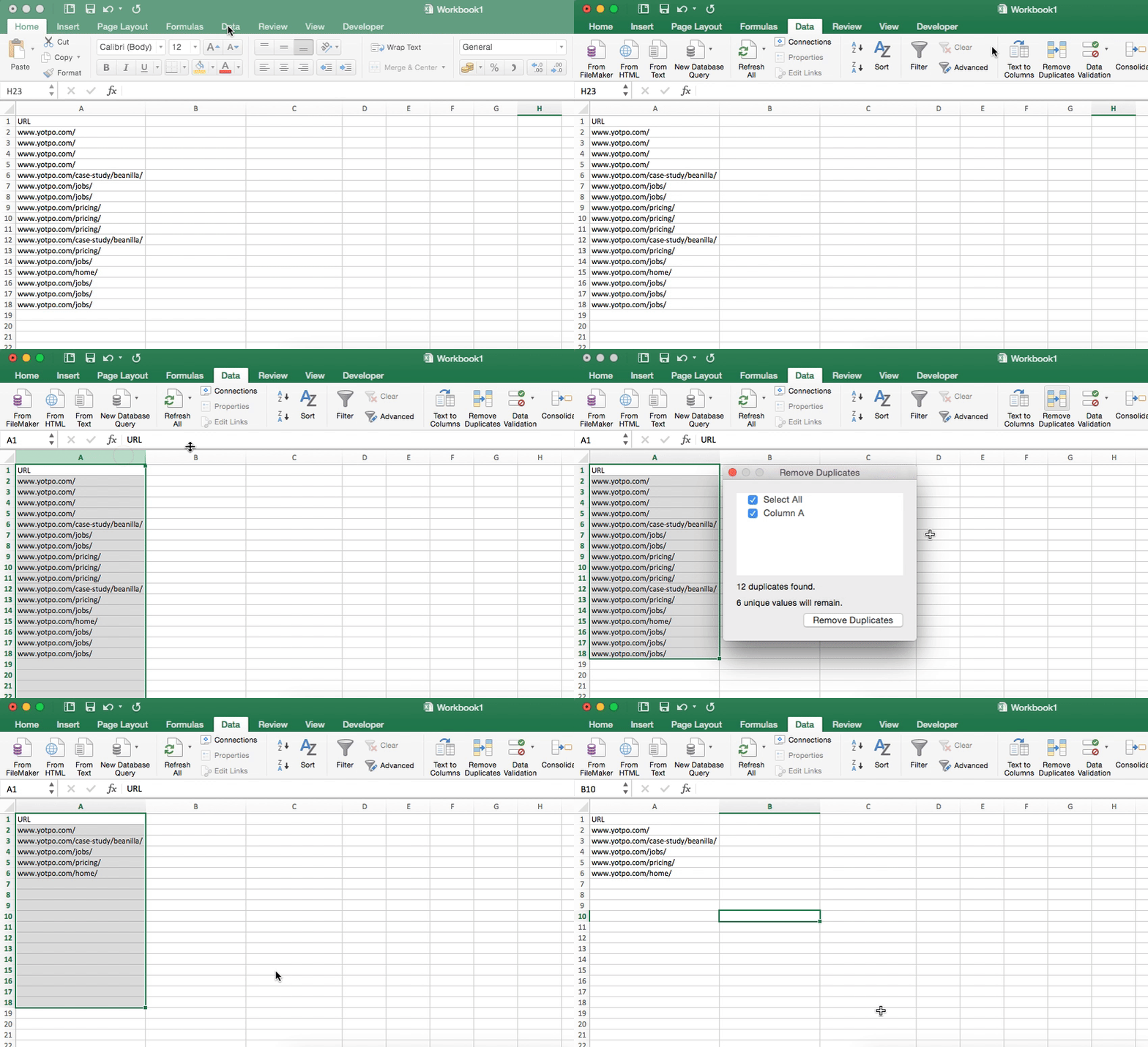
Remove Duplicates is ideal for when you have a large list of data in which some values are repeated (for example, an email list), and you want only one of each value.
How can I use Remove Duplicates?
To use it, go to the “Data” tab, select the column you want to clean up, and click “Remove Duplicates.”
Excel Trick 4: Conditional Formatting
This function allows you to highlight cells or change their color in your Excel sheet based on their value.
When should I use Conditional Formatting?
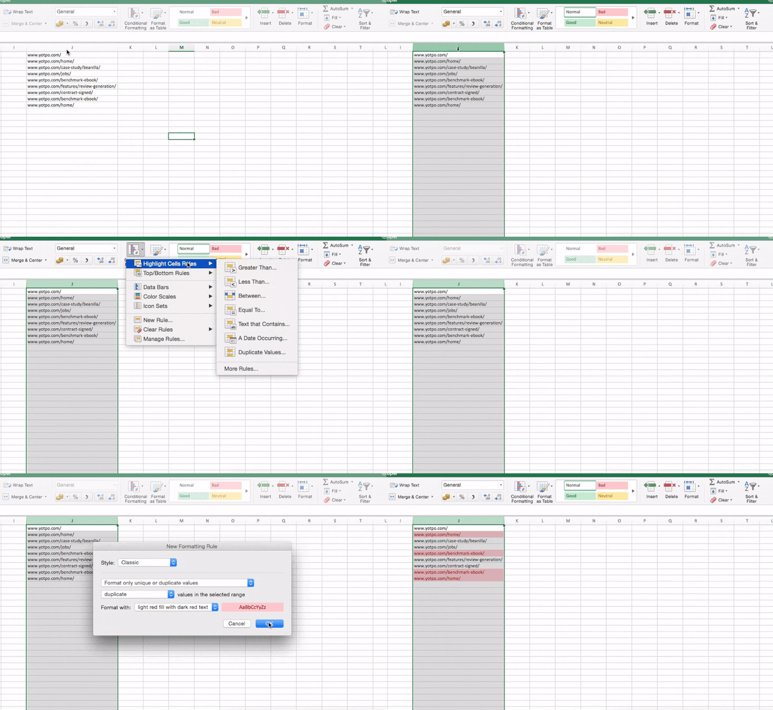
This trick is most helpful for when you need to highlight duplicate values or create a heat map of values. For example, when you have traffic data and you want to see at a glance which page brings the most traffic.
How can I use Conditional Formatting?
To use it to highlight duplicates, select the column you want to format, click “Conditional Formatting” in the top pane, go to “Highlight Cells Rules” and select “Duplicate Values.”
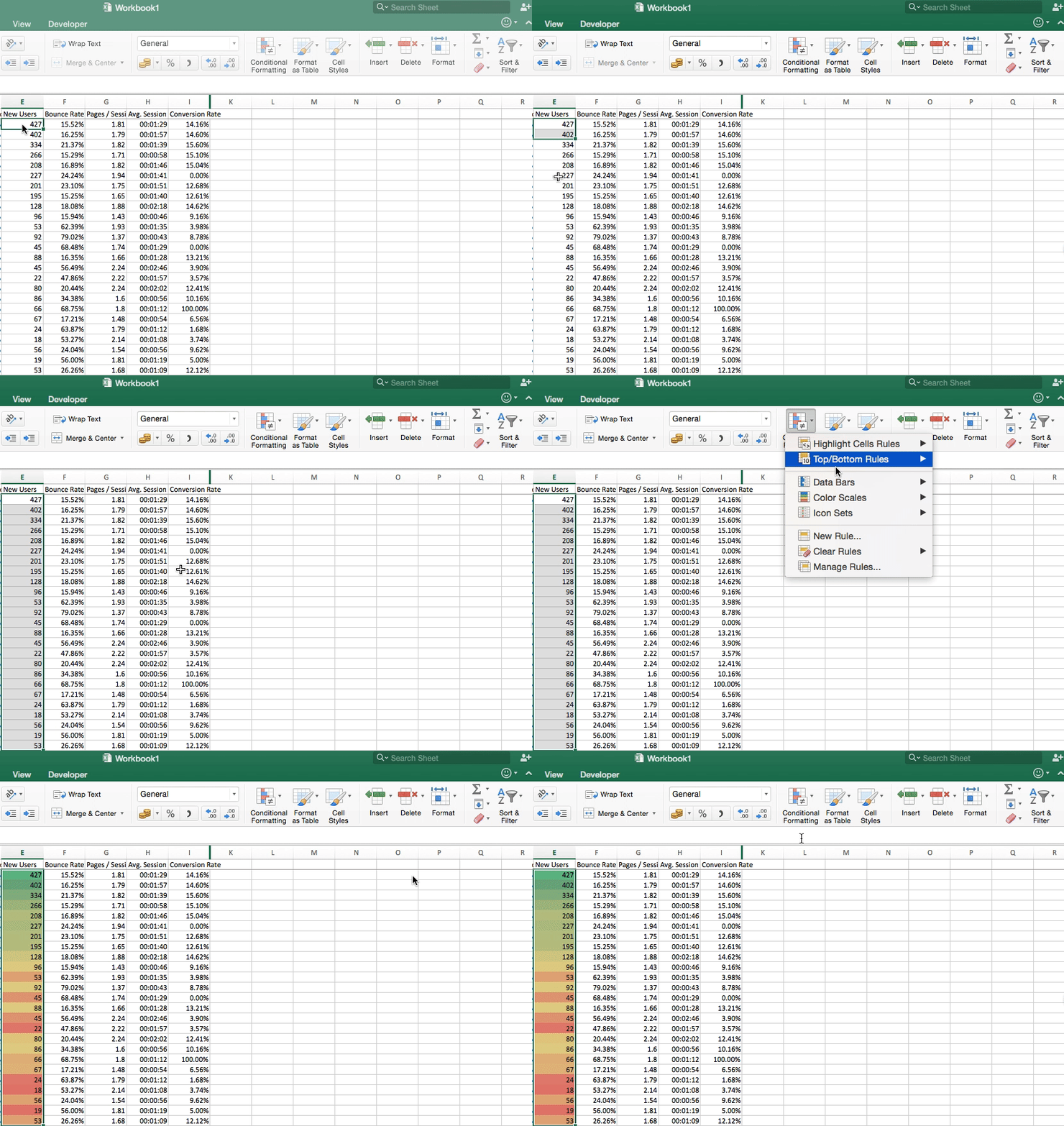
If you’re comparing a lot of different values (for example, looking at the CTR on 100 different emails) you can create a heatmap with Conditional Formatting that will make your best or worst results pop out immediately.
To do this, highlight the column you want to heatmap, select “Conditional Formatting,” select “Color Scales” and pick any of those options.
Excel Trick 5: Paste Special
There are a few Paste Special options that many people don’t take advantage of.
When should I use Paste Special tricks?
Paste Special can help you when you have too many formulas and your Excel is slowing down. It can also help you if you want to hide formulas.
How can I use Paste Special tricks?
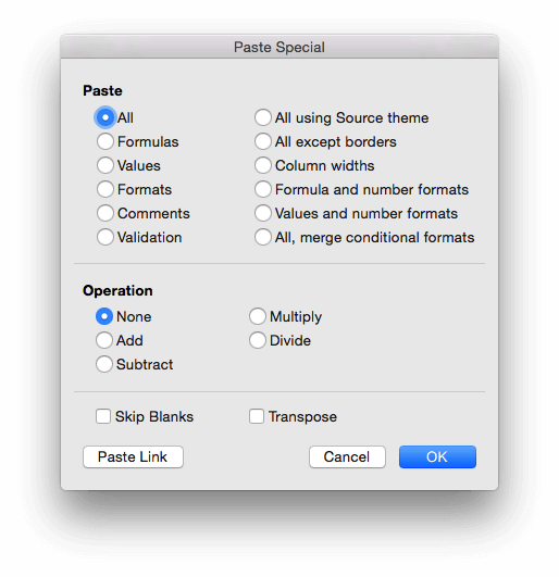
- Formulas: This pastes only the formulas of the copied content.
- Values: One of my personal favorites, this pastes only the values, with no formatting or formulas.
- Formats: This pastes only cell formatting of the copied cells.
Another interesting option here is “Transpose,” which changes the columns of the copied data to rows and vice versa.
Excel Trick 6: Remove blanks
Few people know about this trick, but it is crucial when you’re dealing with a lot of Excel data.
When should I remove blanks?
Let’s say you have an email list with tons of blanks, in this case, you can use remove blanks to get rid of them so you can see clean data.
How can I remove blanks?
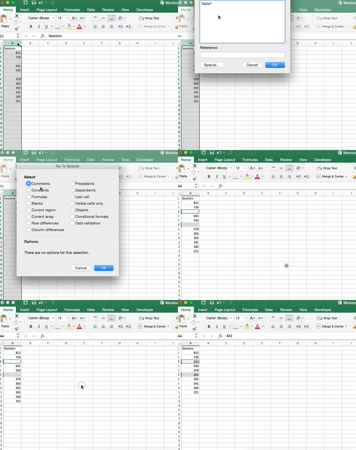
To remove blanks from a column or a row, select the column or row you want to remove blanks from and then press CTRL+G.
This window will appear:
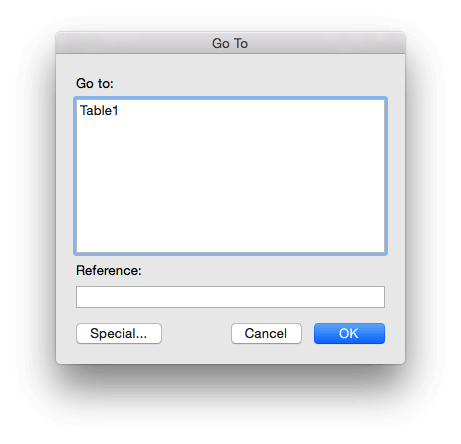
Select “Special,” select “Blanks”, click on CTRL+-, and click “Shift cells up.”
Excel Trick 7: Freeze Panes
The Freeze Panes function locks a certain column or row in your sheet so it can be visible when you scroll.
When should I use Freeze Panes?
Have you ever scrolled so far down an Excel sheet that you forget which column is which? Freeze Panes is for times like these. Freeze Panes can be used to create a sticky column or row that will follow you as you scroll. It’s best for times when you have a big Excel sheet and need to track see data or values from a column or row side-by-side as you scroll.
How can I use Freeze Panes?
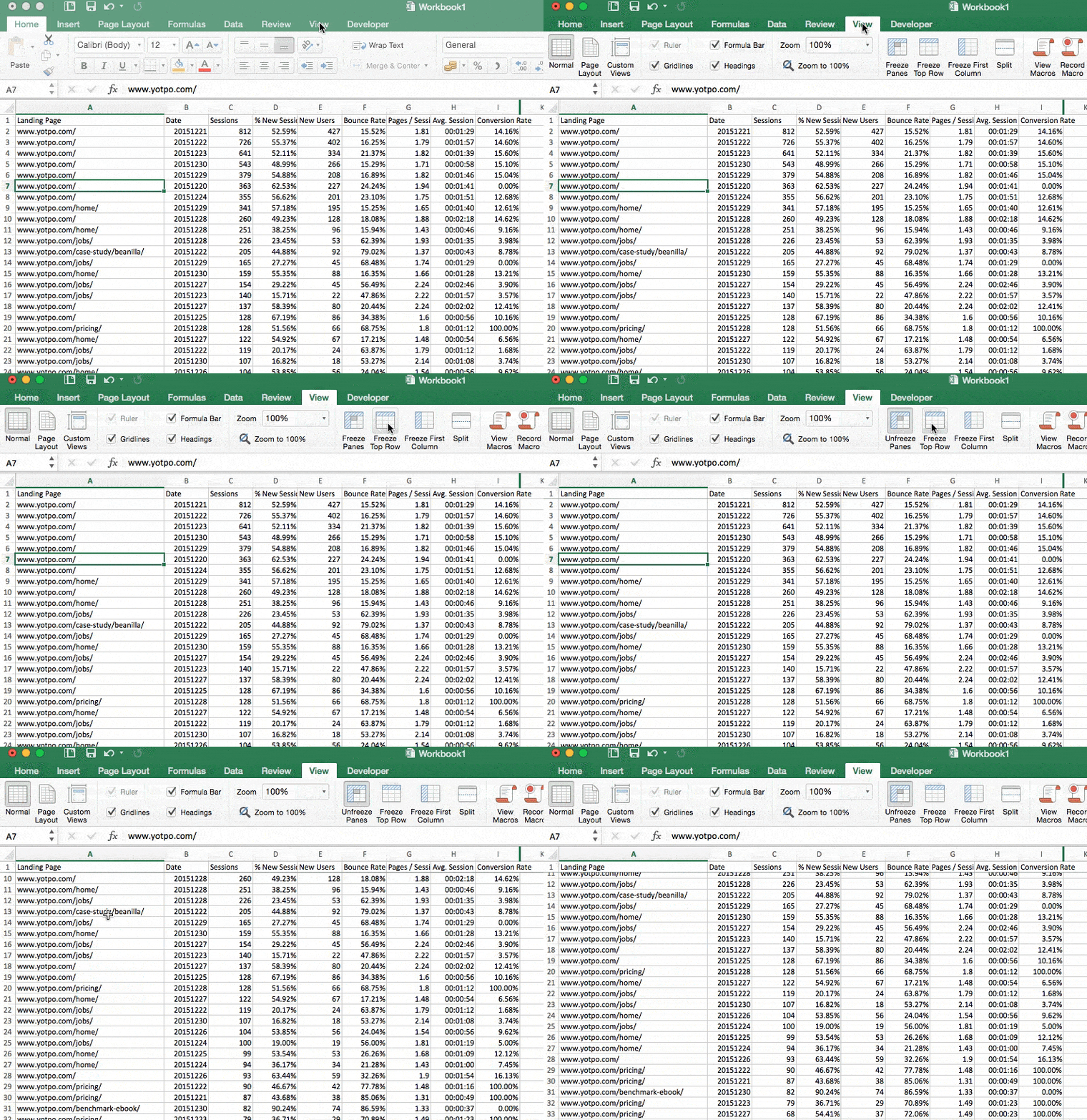
Highlight the column or row you want to freeze. Click to View, and then select “Freeze Top Row.” This will allow you to see the top row no matter how much you scroll.
You can also choose “Freeze First Column” if you want to see the values in a column as you scroll.
Excel Trick 8: Sparklines
Sparklines in Excel are tiny charts that help you show trends in a series of values.
When should I use Sparklines?
Sparklines allow you to visualize trends for small amounts of data.
How can I use Sparklines?
To use Sparklines, highlight the row or column you want to show the Sparklines for, Insert > Sparklines > Lines, pick the cell.
To add color to make the Sparklines pop, go to Sparkline Design in the menu, click marker color, and select the color you want.

Excel Trick 9: Dollar Sign
The Dollar Sign is used to anchor a cell range in a function.
When you normally copy and paste Excel functions, the functions are copied relatively – the dollar sign anchors specific cells so that the function would relate to the cells themselves and not their relative position.
When should I use Dollar Sign?
An example of when this trick can be helpful is if you want to look at a Run Rate. You can dollar sign the cell with the number of days so you can divide the number by a set of cells (rather than the values in the entire row or column).
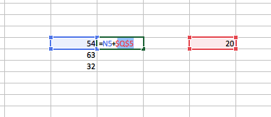

In the above example I added the value of the right cell to the list on the left using the dollar sign.
Without the dollar sign:

The value will be determined by the relative position of the cell.
Excel Trick 10: Grouping
Grouping is great for when you’re looking at large data tables and want to group different pieces of data together.
When should I use Grouping?
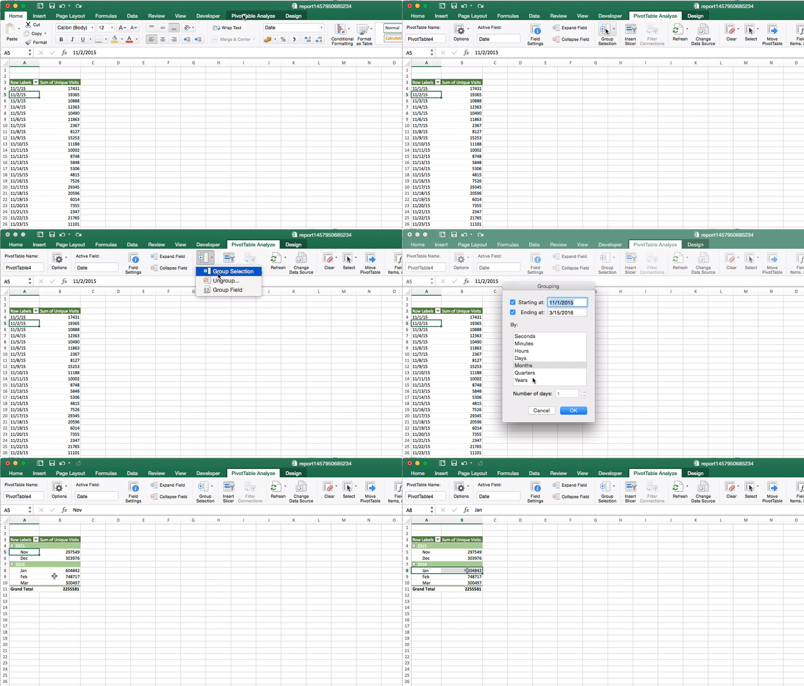
Let’s say you have a lot of dates and you want to see all the days in a month grouped together. In this case, you can group the data by month rather than trying to manually add it up.
How can I use Grouping?
Select the row or column you want, go to PivotTable Analyze in the menu, go to Group Selection, select the row or column you wnat to group and how you want it grouped and wahlah
Conclusion
There you go – our top picks for easy Excel tricks that can make you a more effective marketer. Do you have any other tips to add? We’d love to hear – share your tricks in the comments below.










 Join a free demo, personalized to fit your needs